The goal of this notebook to compute terrain lighting using web map terrain tiles as input and produce corresponding raster light maps as output. For terrain data, we’ll be using the excellent and open Mapterhorn tileset. We’ll start with a simple horizon visibility algorithm and extend it to cover self-shadowing and ambient occlusion. It’s definitely not novel, but the devil is in the details.

Although I don’t work in mapping anymore, I’ll always have have a soft spot for experimental map rendering techniques. Previously I’ve built a live solar terminator map and a kinda janky 3D map renderer. Inspired by some good posts on the topic, I’ve also dabbled in heightfield shadowing. This article finally pulls the latter work together into something functional.

Inspiration

First of all, the best resource on the topic is Tom Patterson’s shadedrelief.com. Any work in map shading can only aspire to convey topography and tell stories in the way his maps do. Alas, I’ve set myself up to fail in the shadow of such a behemoth. But at any rate, my goal is somewhat focused here, to shade map tiles for real time interactive usage.

Next is shadowmap.org. It’s an excellent product for precise map shadowing. As best as I can tell, they use standard z-buffer shadow mapping techniques to compute shadows, but they do it quite well. Whatever the pros and cons, my interest is different, to compute light maps as raster tiles.

One approach for heightfield shading is to shoot rays. Rye Terrell’s terrain shading marches rays from each pixel along the surface and in the direction of the sun, checking for occlusion along the way. The results are beautiful, but the cost is high and it suffers from tile-boundary discontinuities which Terrell addresses by brute-force rendering 3×3 tiles (768×768) and extracting the center.

A cheaper alternative is to sweep across the grid, tracking horizon visibility in a stack. Karim Naaji’s Line-Sweep Ambient Occlusion sweeps rows of the grid, tracking visibility and applying shading in a single pass. However, the technique is limited to eight cardinal directions and still suffers from tile boundary discontinuities.

This article doesn’t offer fundamentally new insight but instead builds on and extends the line-sweep idea to address its shortcomings. In particular it extends the line-sweep to arbitrary directions, uses geometric shadowing to produce soft shadows, and avoids tile boundary discontinuities by prewarming horizon visibility with parent tile data.

Line-sweep horizon visibility

The core primitive behind this notebook is a 1-D sweep that tracks the upper convex hull of elevations seen so far along each ray. Imagine sweeping along a single slice of terrain elevations. As the sweep advances left to right, we test each new point to see if it’s a horizon. If we step uphill far enough that multiple horizons become visible, we pop horizons off of the stack until exactly one horizon remains visible.

Self-shadowing

From here, it’s only a small step farther to compute self-shadowing. At each point during the sweep, we compare the horizon angle to the sun angle. If the sun is below the horizon, the terrain is shadowed.

A particularly nice feature of this algorithm is that we can compute horizon visbility and lighting in the same pass. Neglecting the depth of the stack which generally remains quite small, the algorithm is O(n) in terrain data resolution, requiring that we read each terrain value only once. I can’t immediately see that we could do significantly better.

A little more work is necessary before we can apply this to terrain tiles. The algorithm so far presumes that we’re sweeping along a well-defined grid direction. We’d like to be able to compute shadowing in arbitrary directions.

The solution is simple but requires some finesse. The diagram below illustrates grid traversal in arbitrary directions. We start our first sweep in the upper left corner, seeding subsequent sweeps with remaining pixels along the left edge. For each sweep, we step rightward exactly one pixel and upward by a fractional amount. Once we’ve exhausted all sweeps starting along the left edge, we step rightward along the bottom edge with a given stride, performing identically the same sweeps from the new seed points.

This sequence only handles sweep angles in a single octant of the possible Drag the handle below and observe that for other octants, we simply flip and rotate our canonical octant. In practical terms, this can be implemented with ndarray-style index arithmetic.

One subtlety is that rays pass between integer pixel rows. We can easily distribute values between adjacent pixels using linear interpolation. Where the rubber really meets the road though is that when we layer the sweep algorithm on top of this, we have to be quite careful about positioning, lest we inaccurately compute the terrain slope and create spurious shadows.

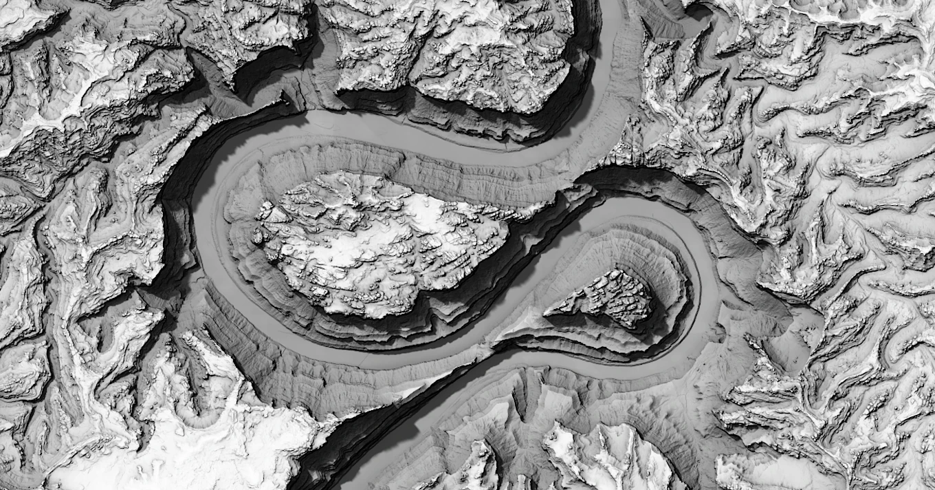
The challenges can be overcome though, and the figure below illustrates the result. Drag the handle and observe that the terrain tile correctly casts shadows on itself.

Soft shadows

We’ve been considering hard thresholds, but we’re well poised to relax this to a smooth threshold so that we can emulate the soft penumbra of a finite-sized light source like the sun. Realistically, the sun covers about degrees in the sky, making it pretty close to a point source, but we can always increase the size for visual effect.

The figure below illustrates a soft shadowing pass using a smoothstep function for horizon visibility occlusion.

Sadly though, the sun is a two-dimensional source, and we’ve only discussed softening in one dimension. Short of something fancy like mipmaps, all I was able to come up with was to naively average multiple samples of our altitude-wide analytical soft shadows across the azimuthal direction.

Samples aren’t cheap, so it’s worth thinking carefully about how to distribute samples across the sun disk. Our altitude-wise analytical soft shadows use a smoothstep function, so after some consideration, I scaled a Gaussian function to roughly approximate the smoothstep function, then distributed equally-weighted samples in the azimuthal direction using inverse-CDF sampling to approximate the desired Gaussian.

The sun isn’t really a Gaussian disk, of course. But Gaussians are mathematically separable, which makes the 1D altitude × 1D azimuth factorization work out cleanly, and the resulting penumbra looks smooth enough in practice that the approximation pays off.

Parent-tile pre-pass

A limitation of per-tile methods is that they have no knowledge of terrain beyond their edges. External mountains which would cast shadows onto the tile are not considered, producing visible seams between tiles. A natural solution is to use lower-resolution parent tile data to build a horizon stack before sweeping across the computation tile.

In fact we can step multiple levels upward in the tile pyramid to further extend the range of this pre-warming. A 2×2 block of parents physically covers tile widths around the computation tile. Thus, a 2×2 block of parent tiles always covers a 3×3 area relative to zoom , while grandparent tiles cover a 5×5 area, and tiles a 9×9 area.

In practice, seems a reasonable tradeoff, and we can use the maximum possible projected shadow length to limit the extent of the pre-pass horizon visibility sweep. That is, when the sun is directly overhead, shadows are very short and we don’t need to march all the way to the edge of parent to know that features there could not possibly cast a shadow onto the computation tile.

Toggle the parent-tile pre-pass below and observe its effect in the vicinity of tile boundaries. The selector shows how the covered-area / resolution trade plays out visually — at the comp-tile red outline shrinks to of the horizon width (4× the surrounding area captured), and at to . Dragging the sun handle upward also shrinks the blue “horizon touched” tint toward the tile — you’re watching the elevation-bounded trim kick in.

Line-sweep ambient occlusion

The same horizon visibility sweep works for ambient occlusion as well. Ambient occlusion proceeds similarly to shadowing, but instead of illumination by a point source, each pixel is illuminated by the portion of sky visible to it. I extended Karim Naaji’s LSAO to support parent-tile occlusion and arbitrary sweep directions. That leaves one design knob open: the per-slice visibility function that maps each swept horizon angle to a shade contribution.

Naaji uses . The function drops with slope right at , so even a shallow horizon produces an immediate darkening. The tradeoff is a long tail, so distant tall features keep contributing, and tile boundaries take extra care.

A Lambertian sky integral offers a physically motivated alternative. Incident sky radiance from a direction at zenith angle is weighted by , so the visible fraction of one azimuthal slice above a horizon at elevation α is

which normalises to : 1 at a flat horizon, 0 at a vertical wall. Its slope is flat at and steepens later, giving a softer, more forgiving response to small horizons. And because for small α, distant tall blockers fall off as , so the effect is strongly local and tile boundaries are less visible.

Honestly though, I think the particular choice of function is best thought of as an artistic decision. The original function seems to produce better visual separation of features at the cost of less locality.

In practice, we use a Web Worker pool to compute independent sweeps, then average them to compute pixel value . For display, a contrast slider tone-maps the response. For pixel , an tonemap squashes the scaled shade into :

Relief shading

Lit surfaces vary in brightness depending on their orientation. The most natural lighting choice is diffuse Lambertian shading, but this tends to darken the surface when lit at oblique angles, which isn’t necessarily what we want for a map.

Relief shading separates the terrain slope from its aspect (direction it faces relative to the sun), so the sun’s altitude doesn’t darken flat ground. Flat terrain stays white, slopes facing the sun brighten, and slopes facing away darken. Strength of the effect is proportional to the slope angle.

Concretely, I’ve adapted GDAL’s relief shading function, computing the slope angle and the aspect alignment , then a darkness term where is the strength parameter. The final relief value is . The z-factor (where is the sun’s altitude) dampens slopes following the GDAL convention and modulates the perceived slope by sun altitude.

Zoom-dependent gradient attenuation

One annoyance is that shading fades at low zoom. Peaks survive downsampling well, but decimation reduces the gradient and fails to commute with nonlinearities in the shading function.

A quick check across a handful of Mapterhorn tiles suggests a rough power-law attenuation of average elevation gradient, so we reduce the horizontal grid spacing at low zoom to steepen gradients and leave shading visually similar in appearance.

This is one thing I’m not content with since I’d prefer a physicaily accurate function which does not need a correction factor. The map on this page uses tiles of the same zoom, but tiles with different zooms, like on a pitched 3D map, would show discontinuous shading due to this inconsistency.

WebGPU implementation

From the start, I was pretty excited about the implementing this in a WebGPU compute shader. It’s perfectly set up for it, where each scanline sweep is an independent thread. This is similar to Rye Terrell’s appraoch described above, except that it’s a compute shader so that we can shade as we traverse!

In the end though, it contends with GPU resources and does not appear to work very well, slowing down the map interface as tiles are computed. The figure below illustrates successful computation in WebGPU, but th efinal renderer favors a CPU worker pool for lighting computation.

Live WebGPU tile viewer

Finally, we have all the pieces in place to produce a map. In the map below, each tile goes through a two-phase bake (CPU or GPU). The static bake runs once when the tile’s elevation data arrives: compute surface normals, 8-pass LSAO, and pack the results into an rgba8unorm texture:

The shadow re-bake runs whenever the sun direction changes, packing shadow values into the alpha channel for use in the final shading step. We can even use Volodymyr Agafonkin’s suncalc library to compute physically accurate sun angles!

The map viewer below is thrown together hastily with the help of Claude since I was not able to find another viewer which satisfied my requirements. Although it’s not hard to get tiles onto a map, it’s tricky if you really care about tile lifecycle, multi-pass computation, and smooth updates. Pan with click+drag; zoom with the mouse wheel.

Overall, I’m pretty happy with the technique, and at least happy that I probably took this idea and ran with it about as far as one would be advised to do. I wonder if mipmaps would enable soft shadows with a single pass. I’m not sure if it’s performant enough to be practical. And at any rate, if you really want good shadowing, you might just be advised to use more standard shadow map techniques for shadowing.